GatingTree: Analyzing Cytometry Data with GatingTree

1. Loading Libraries and Data

First, load the necessary libraries and download the test data using HDCytoData.

library(GatingTree)
library(HDCytoData)
library(flowCore)
d_SE <- Weber_AML_sim_main_5pc_SE()

This command downloads a hybrid mass cytometry dataset constructed by spiking a small percentage of Acute Myeloid Leukemia (AML) cells into healthy bone marrow cells (Weber et al., 2019).

2. Preprocessing Data

We convert the raw cytometry data into a format suitable for GatingTree analysis by mapping the experiment metadata and filtering relevant markers.

# Extract experiment information and channel names
experiment_info <- d_SE@metadata$experiment_info
channel_name <- colnames(d_SE)

# Prepare sample definitions
sampledef <- experiment_info[, c("sample_id", "group_id")]
colnames(sampledef) <- c('file','group')

# Filter markers based on specific criteria
marker_info <- as.data.frame(d_SE@colData)
logic <- marker_info$marker_class == 'type' | marker_info$marker_name == 'DNA1'
marker_info <- as.data.frame(marker_info[logic,])

# Extract expression data and adjust column names
exprs <- assay(d_SE)
annotationdf <- as.data.frame(rowData(d_SE))
logic <- colnames(exprs) %in% marker_info$channel_name
data <- exprs[, logic]
colnames(data) <- marker_info$marker_name
colnames(data) <- gsub("-", "", colnames(data))
data <- cbind(data, data.frame(file = annotationdf$sample_id))
data <- as.data.frame(data)

# Define variables excluding 'DNA1' and 'file'
cnlogic <- colnames(data) %in% c("DNA1", "file")
variables <- colnames(data)[!cnlogic]
# Remove unnecessary samples
logic <- grepl(pattern = 'CBF', data$file)
Data <- data[!logic,]
# Define sample definitions (grouping) by sampledef
sampledef <- sampledef[!grepl(pattern = 'CBF', sampledef$group),]

2. Creating a FlowObject and Applying Data Transformation

Create a FlowObject using the prepared data and sample definitions.

# Create FlowObject
x <- CreateFlowObject(Data = Data, sampledef = sampledef, experiment_name = 'AML_sim')

We can display the sample grouping using the showSampleDef function:

showSampleDef(x)

##          file   group
## 1  healthy_H1 healthy
## 2  healthy_H2 healthy
## 3  healthy_H3 healthy
## 4  healthy_H4 healthy
## 5  healthy_H5 healthy
## 6       CN_H1      CN
## 7       CN_H2      CN
## 8       CN_H3      CN
## 9       CN_H4      CN
## 10      CN_H5      CN

Next, apply data transformation. A moderated log transformation using the LogData function is recommended to normalize the data:

x <- LogData(x, variables = variables)

4. Determining Positive/Negative Threshold for Markers

Use DefineNegatives to define the negative/positive threshold for each of your variables, activating interactive sessions.

x <- DefineNegatives(x)

Alternatively, you can import predefined thresholds using import_negative_gate_def:

file_path <- system.file("extdata", "negative_gate_def_AML.csv", package = "GatingTree")
negative_gate_def <- read.csv(file_path)
x <- import_negative_gate_def(x, negative_gate_def)

After defining the negative thresholds, inspect the results by visualizing them using PlotDefineNegatives.

To produce density plots (histograms):

x <- PlotDefineNegatives(x, y_axis_var = 'Density', panel = 4)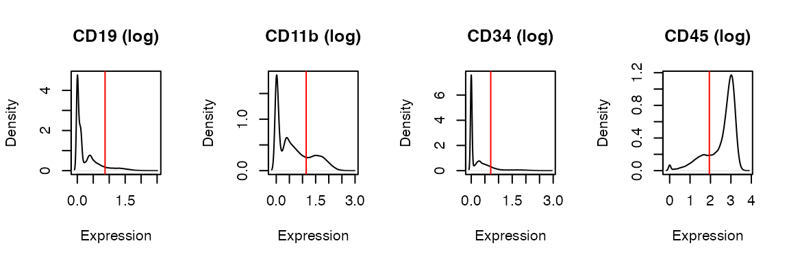

Vertical line (red line) indicates the threshold value.

For 2d plots, choose a variable for y-axis:

x <- PlotDefineNegatives(x, y_axis_var = "CD3.logdata", panel = 4)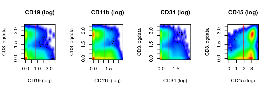

5. Perform GatingTree Analysis and Visualization

With the data prepared and thresholds defined, perform the GatingTree analysis. Use the createGatingTreeObject function to conduct pathfinding analysis in multidimensional marker space and construct a GatingTree.

x <- createGatingTreeObject(x, maxDepth = 5, min_cell_num=0, expr_group = 'CN', ctrl_group = 'healthy', verbose = FALSE)

Visualize the GatingTree output:

x <- GatingTreeToDF(x)
node <- x@Gating$GatingTreeObject
datatree <- convertToDataTree(node)
graph <- convert_to_diagrammer(datatree, size_factor=1, all_labels = F)

library(DiagrammeR)
render_graph(graph, width = 600, height = 600)

If necessary, prune the GatingTree to focus on the most informative nodes:

x <- PruneGatingTree(x, max_entropy = 0.5, min_enrichment=0.5)

Visualize the pruned GatingTree:

pruned_node <- x@Gating$PrunedGatingTreeObject
datatree2 <- convertToDataTree(pruned_node)
graph <- convert_to_diagrammer(datatree2, size_factor=1)
render_graph(graph, width = 600, height = 600)

6. Delta Enrichment Analysis

Finally, assess the impact of adding each marker state to the enrichment score using the PlotDeltaEnrichment function.

x <- PlotDeltaEnrichment(x)

##   Kruskal-Wallis rank sum test
## 
## data: x and group
## Kruskal-Wallis chi-squared = 181.6968, df = 31, p-value = 0
## 
## 
## alpha = 0.05
## Reject Ho if p <= alpha/2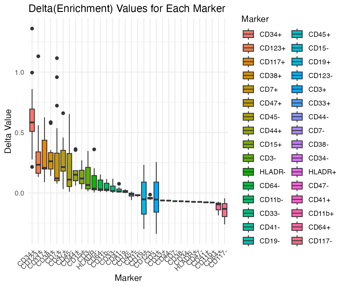

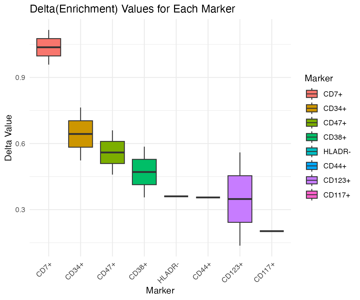
PlotDeltaEnrichmentPrunedTree further clarifies the impact of important markers using Pruned Gating Tree.

x <- PlotDeltaEnrichmentPrunedTree(x)

##   Kruskal-Wallis rank sum test
## 
## data: x and group
## Kruskal-Wallis chi-squared = 9.625, df = 9, p-value = 0.38
## 
## 
## alpha = 0.05
## Reject Ho if p <= alpha/2