TockyPrep: Data Preprocessing Methods for Flow Cytometric Fluorescent Timer Analysis
Dr. Masahiro Ono
2025-02-08
Source:vignettes/TockyDataPreprocessing.Rmd
TockyDataPreprocessing.Rmd

Introduction
TockyPrep: Standardizing the Analysis of Fluorescent Timer Proteins in Flow Cytometry
Fluorescent Timer proteins uniquely change their emission spectra over time and serve as powerful tools for monitoring the dynamic processes within cells. These proteins are crucial for understanding the intricate temporal dynamics of cellular events. Despite their potential, the analysis of Timer fluorescence data in flow cytometry is often complicated by variability in instrument settings and the absence of standardized data preprocessing methods. To overcome these challenges, the TockyPrep package has been developed. This R package provides a comprehensive suite of tools designed to automate the preprocessing, normalization, and trigonometric transformation of Timer fluorescence data.
Aim
The TockyPrep package aims to standardize the analysis of Timer fluorescence to improve reproducibility and accuracy across various experimental setups. It specifically addresses the normalization of immature and mature Timer fluorescence as a critical step for robust analysis. This approach is central to understanding the maturation dynamics of Timer proteins, and is implemented using advanced trigonometric transformations.

Getting Started with TockyPrep
To begin using TockyPrep, install the package from GitHub using the following command:
# Install TockyPrep from GitHub
devtools::install_github("MonoTockyLab/TockyPrep")
Once installed, you can load the package and follow the vignette’s sample workflow to process your flow cytometry data. This vignette will guide you through importing your data, applying preprocessing steps, and visualizing the results to ensure that you can fully leverage the capabilities of the TockyPrep toolkit.
Sample Workflow
This section will walk you through a typical analysis workflow using TockyPrep to process flow cytometric data of cells expressing Fluorescent Timer proteins. We will cover data import, application of preprocessing methods, and basic visualization techniques.
Set-up and prep_tocky
To start the TockyPrep analysis, load the library.
We will use example files included in the TockyPrep package. To access the files, run the following codes, which defines the sample files and the negative control file to be used.
# Example data load
# Define the base path
file_path <- system.file("extdata", package = "TockyPrep")

# Define files
negfile <- "Timer_negative.csv"
samplefiles <- list.files(file_path, pattern = "sample_", full.names = FALSE)
samplefiles <- setdiff(samplefiles, file.path(file_path, negfile))


print(negfile)
## [1] "Timer_negative.csv"
head(samplefiles)
## [1] "sample_0hrs_R1.csv"  "sample_0hrs_R2.csv"  "sample_0hrs_R3.csv"
## [4] "sample_12hrs_R1.csv" "sample_12hrs_R2.csv" "sample_12hrs_R3.csv"
We will define the files to be analyzed using the function
prep_tocky.
# Preprocessing data
prep <- prep_tocky(path = file_path, samplefile = samplefiles, negfile = negfile, interactive = FALSE)
Data preprocessing by timer_transform
Now we are ready to apply the data preprocessing methods to the
sample data. timer_transform does all the steps,
including the data import, Timer thresholding, Timer
fluorescence normalization, and Trigonometric transformation to
obtain Timer Angle and Intensity values for individual cells.
# Normalizing and transforming data
transformed_data <- timer_transform(prep, blue_channel = 'Timer.Blue', red_channel = 'Timer.Red', select = FALSE, verbose = FALSE)

Visualization
Preparation: sample grouping definition
To effectively visualize the processed data, sample grouping
needs to be defined using sample_definition. The
example file sampledefinition.csv provides the
standard form. Use data.frame as input into
sample_definition.
sample_definition <- read.csv(file.path(file_path, 'sampledefinition.csv'))
sample_definition <- as.data.frame(sample_definition)
head(sample_definition)
##                  file group
## 1  sample_0hrs_R1.csv     0
## 2  sample_0hrs_R2.csv     0
## 3  sample_0hrs_R3.csv     0
## 4 sample_12hrs_R1.csv    12
## 5 sample_12hrs_R2.csv    12
## 6 sample_12hrs_R3.csv    12
# Normalizing and transforming data

transformed_data <- sample_definition(transformed_data, sample_definition = sample_definition, interactive = FALSE)
Alternatively, sample grouping can be created by choosing
interaction session using the option
interactive = TRUE. This will prompt generation
of sample_definition.csv in your output directory.
Confirming the gating of Timer fluorescence
To visualize the thereshold values for Timer blue and red
fluorescence, use plot_timer_gating.
plot_timer_gating(prep = prep, x = transformed_data)
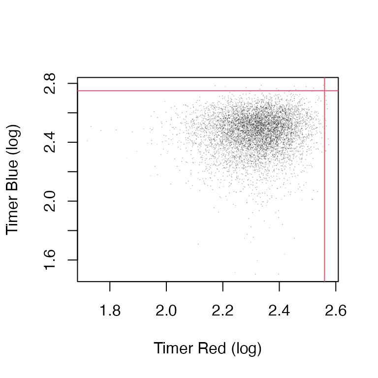
Figure 1: Thereshold values set for Timer blue and red fluorescence.
## Percentage of cells in each quadrant:
## Q1: 0.2029%
## Q2: 0%
## Q3: 0.2029%
## Q4: 99.5941%
Visualization of the processed Timer data
To visualize the processed Timer data, use
plot_tocky. This is a versatile function,
enabling the three plot modes, including
'Timer fluorescence',
'Normalized Timer fluorescence', and
'Timer Angle and Intensity'.
-
'Timer fluorescence': Timer blue and red fluorescence, without normalization. -
'Normalized Timer fluorescence': Normalized and thrsholded Timer blue and red fluorescence. -
'Timer Angle and Intensity': Timer Angle and Intensity after trigonometric transformation.
Non-normalized Timer fluorescence (Figure 2)
The default is 'Timer fluorescence', which is
non-normalized Timer fluorescence.
logic <- sample_definition$group %in% c(4, 8, 12, 16)
samplefiles <- sample_definition$file[logic]
show(samplefiles)
##  [1] "sample_12hrs_R1.csv" "sample_12hrs_R2.csv" "sample_12hrs_R3.csv"
##  [4] "sample_16hrs_R1.csv" "sample_16hrs_R2.csv" "sample_16hrs_R3.csv"
##  [7] "sample_4hrs_R1.csv"  "sample_4hrs_R2.csv"  "sample_4hrs_R3.csv"
## [10] "sample_8hrs_R1.csv"  "sample_8hrs_R2.csv"  "sample_8hrs_R3.csv"
# Visualizing the results
plot_tocky(transformed_data, interactive = FALSE, save = FALSE, n = 2, samplefile = samplefiles, verbose = FALSE)
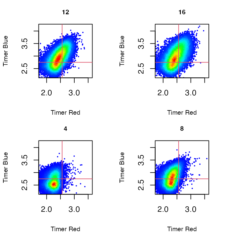
Figure 2: Non-normalized Timer Fluorescence in T cells stimulated by antigen and analyzed at 4, 8, 12, and 16 hours after activation.
Normalized Timer fluorescence (Figure 3)
Using the option
plot_mode = "Normalized Timer fluorescence", you
can visualize Normalized Timer blue and red fluorescence.
# Visualizing the results
plot_tocky(transformed_data, plot_mode = "Normalized Timer fluorescence", interactive = FALSE, save = FALSE, n = 2, samplefile = samplefiles, verbose = FALSE)
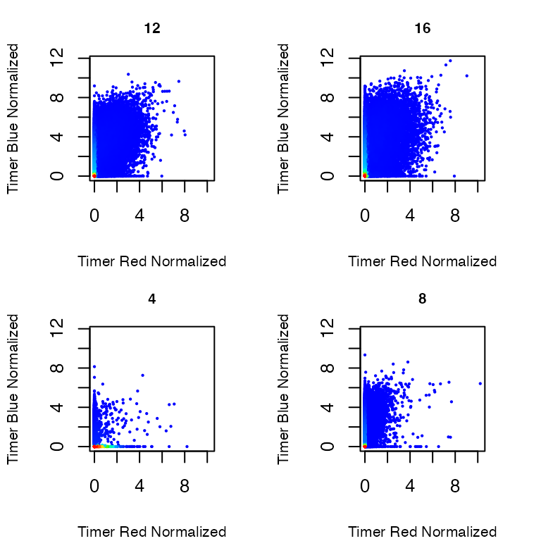
Figure 3: Normalized Timer Fluorescence in T cells stimulated by antigen and analyzed at 4, 8, 12, and 16 hours after activation.
Timer Angle and Intensity (Figure 3)
Using the option
plot_mode = "Timer Angle and Intensity", you can
visualize the effects of the trigonometric transformation
applied to the normalized data.
# Visualizing the results
plot_tocky(transformed_data, plot_mode = "Timer Angle and Intensity", interactive = FALSE, save = FALSE, n = 2, samplefile = samplefiles, verbose = FALSE)
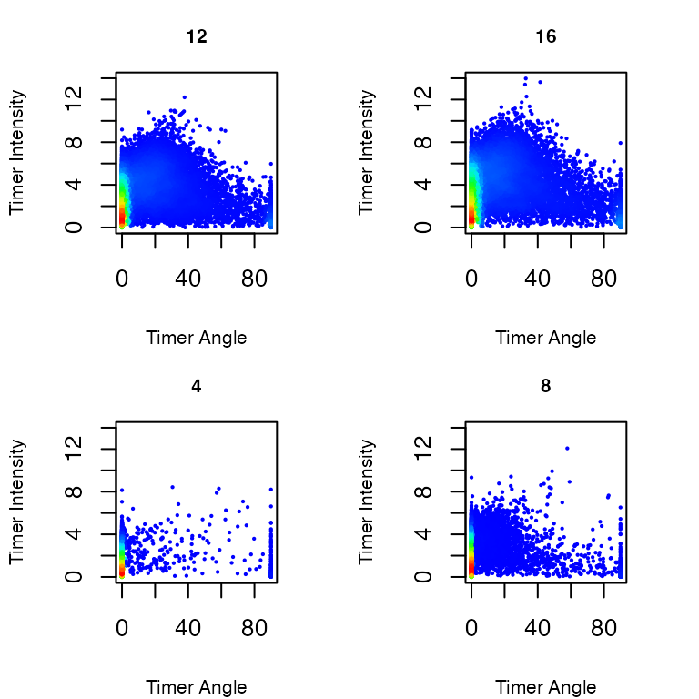
Figure 3: Timer Angle and Timer Intensity in T cells stimulated by antigen and analyzed at 4, 8, 12, and 16 hours after activation.
Exploring Timer Data Transformation Parameters (Figure 4)
Using the function explore_timer_transform, you can
explore the parameter space by varying parameters for Timer
fluorescence normalization and transformation.
explore_timer_transform(prep, transformed_data)
This will activate a Shiny server, allowing you to experiment with changing Timer fluorescence thresholds and different normalization methods.
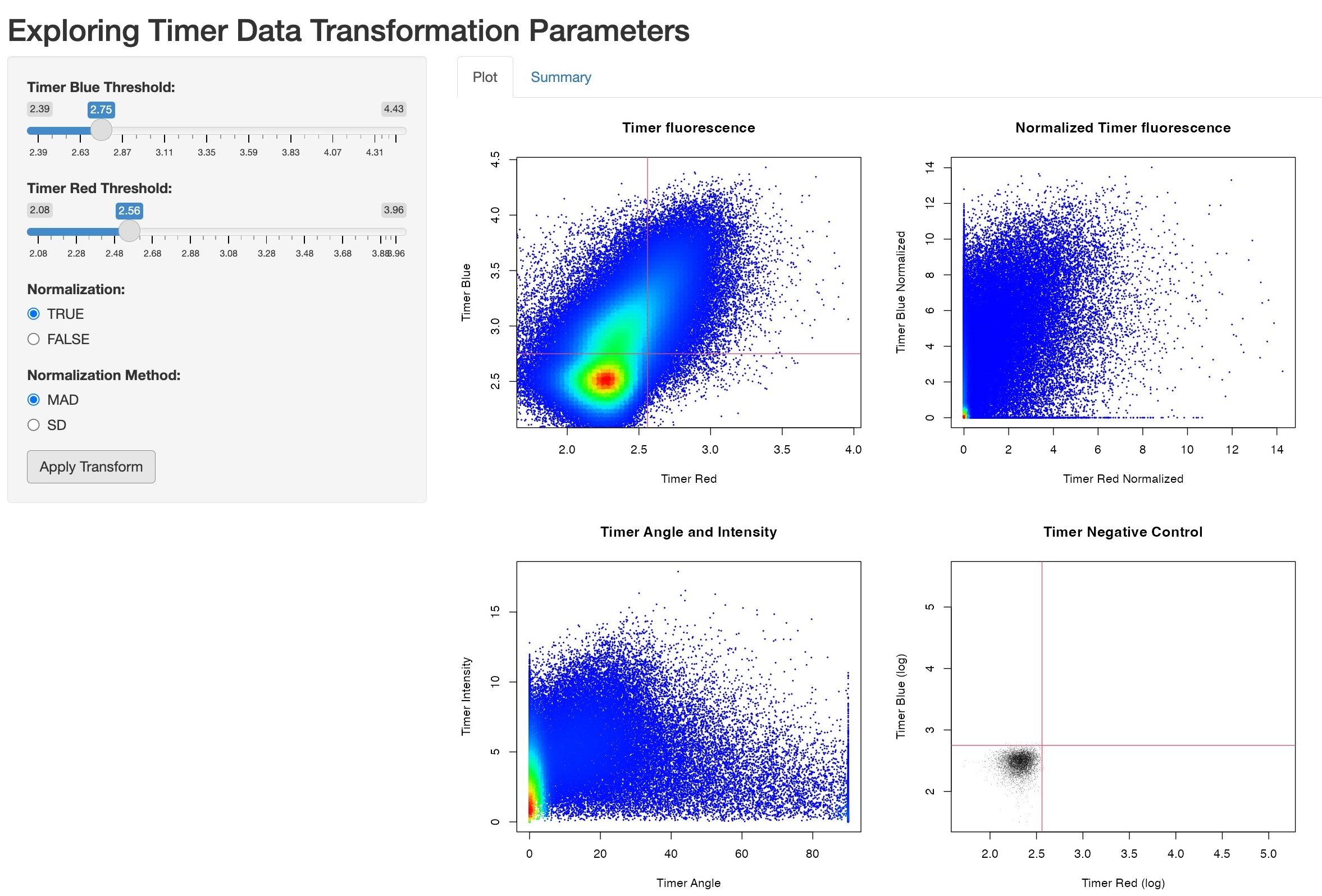
Figure 4: Screenshot of the Shiny Demonstration for Exploring Timer Data Transformation Parameters.
Conclusion
TockyPrep provides a comprehensive suite of data preprocessing methods for deriving Timer Angle and Timer Intensity data. This suite includes Timer thresholding, Timer normalization, and trigonometric transformation. The resulting Timer Angle and Intensity data can be robustly used in downstream analyses.
Please explore downstream analysis examples in Bending, Martı́n, et al. (2018); Bending, Paduraru, et al. (2018); and Hassan et al. (2022).

